A simple word game - guess a 5-letter word in six tries. Wordle, created by Josh Wardle, quietly turned into a daily habit for thousands of people — so much so that the New York Times ended up buying it for at least a million dollars.
Like many others, I got into the habit of looking up the meaning of the day’s word — especially when it wasn’t something I’d normally use. At some point, I wondered: if this is my instinct, surely others are doing the same?
That led to a small hypothesis, and eventually, a full dataset exploration.
🧠 Hypothesis
Each Wordle word generates a noticeable spike in Google searches on the day it appears — especially if the word is uncommon.
If this is happening at scale, we should be able to observe it using publicly available data.
🔍 What Data We Used
To explore this, I gathered data for each Wordle day including:
Date
Wordle Answer (Source: YourDictionary, from June 2021 – June 2025)
Commonality of the word
Google search trends for that word
We defined commonality using two metrics:
Wordfreq (Python library) – Based on books, websites, etc.
SUBTLEX (Subtitle-based frequency dataset) – Reflects more spoken-word usage
Word Commonality
We used the following formula to normalize commonality:
The max frequency for commanality using wordfreq is based on the word “the”, considered one of the most common words in English.
Show commonality generation code
importmathimportpandasaspdfromwordfreqimportword_frequency# Source: https://www.ugent.be/pp/experimentele-psychologie/en/research/documents/subtlexus (Zipped text version)
_SUBTLEX_SOURCE_PATH='./data/SUBTLEXus.tsv'defsubtlex_commonality(word:str,source_dataset:str='./data/SUBTLEXus.tsv',log_scale:bool=True)->float:word=word.lower()subtlex_df=pd.read_csv(source_dataset,sep='\t')row=subtlex_df[subtlex_df['Word'].str.lower()==word]ifrow.empty:return0.0# Word not found
freq=float(row.iloc[0]['SUBTLWF'])max_freq=subtlex_df['SUBTLWF'].max()iffreq==0ormax_freq==0:return0.0iflog_scale:score=math.log1p(freq)/math.log1p(max_freq)else:score=freq/max_freqreturnround(score,4)defwordfreq_commonality(word:str,lang:str='en',wordlist:str='best',log_scale:bool=True)->float:"""
Returns a commonness score between 0 and 1 based on wordfreq.
Parameters:
- word: the input word to evaluate
- lang: language code (e.g., 'en' for English)
- wordlist: 'best', 'large', 'small' — which corpus group to use
- log_scale: whether to apply log scaling to frequency
Returns:
- A float between 0 (rare) and 1 (very common)
"""freq=word_frequency(word.lower(),lang,wordlist=wordlist)iffreq==0:return0.0iflog_scale:# Use log1p to normalize and smooth
max_freq=word_frequency('the',lang,wordlist=wordlist)# Approx. highest
score=math.log1p(freq)/math.log1p(max_freq)else:# Just scale linearly to "the"
max_freq=word_frequency('the',lang,wordlist=wordlist)score=freq/max_freqreturnround(score,4)defappend_word_commonality(source_dataset:str,fn:callable)->None:"""
Appends the commoness indicator column for each word of the CSV file.
Parameters:
- source_dataset: Path to the dataset to read.
- fn: Function to use for finding the word commoness
"""df=pd.read_csv(source_dataset)df['word']=df['word'].str.lower()df[fn.__name__]=df['word'].apply(fn)df.to_csv(source_dataset,index=False)if__name__=='__main__':print("Starting execution...")source_file='./data/raw_data.csv'append_word_commonality(source_dataset=source_file,fn=wordfreq_commonality)append_word_commonality(source_dataset=source_file,fn=subtlex_commonality)print("Finished execution...")
In this post, unless otherwise noted, we use the SUBTLEX-based commonality score (since I found this to be a better representation).
Google Search Trends
For each word, we queried Google Trends and captured:
Global search volume on the Wordle day
Global average for the previous 200 days
Search volume (on Wordle day) in the “Language Resources” category
200-day average in the same category
Show trend generation code
importpandasaspdfromfunctoolsimportpartialfrompytrends.requestimportTrendReqfromdatetimeimportdatetime,timedelta# Locally would have to update _get_data method's parameter `method_whitelist` to `allowed_methods`
# to work with newer versions of urllib3
pytrends=TrendReq(hl='en-US',tz=360,retries=2,backoff_factor=0.2)defget_trends_usage(word:str,target_date:str,category:int=0)->tuple[int,float]:"""
Returns (usage_on_date, avg_prior_200_days) for a given word and date.
Parameters:
- word: search term
- target_date: 'YYYY-MM-DD' format
Returns:
- Tuple: (value_on_day, avg_of_200_days_before)
"""date_obj=datetime.strptime(target_date,'%Y-%m-%d')start_date=(date_obj-timedelta(days=200)).strftime('%Y-%m-%d')end_date=(date_obj+timedelta(days=1)).strftime('%Y-%m-%d')# include target day
# Format: 'YYYY-MM-DD YYYY-MM-DD'
timeframe=f"{start_date}{end_date}"print(f"Searching for trend of {word} in time range: {timeframe}")try:pytrends.build_payload([word],cat=category,timeframe=timeframe,geo='',gprop='')df=pytrends.interest_over_time()ifdf.empty:return(None,None)df=df.reset_index()df['date']=df['date'].dt.date# strip time
value_on_day=df.loc[df['date']==date_obj.date(),word]avg_before=df.loc[df['date']<date_obj.date(),word].mean()print(f"Found values for {word}: value_on_day = {int(value_on_day.values[0])}, avg_200_days: {round(avg_before,2)}")return(int(value_on_day.values[0])ifnotvalue_on_day.emptyelseNone,round(avg_before,2))exceptExceptionase:print(f"Error for {word} on {target_date}: {e}")return(None,None)defsafe_trends_request(row,col1,col2,category):"""
Even if we run multiple times, we want to ensure we trigger only for those words where we are missing the datapoints.
"""# Skip if both values already exist and are not NaN
ifpd.notna(row.get(col1))andpd.notna(row.get(col2)):# print(f"Skipping for current one! {row.get('word')}")
returnpd.Series([row[col1],row[col2]])returnpd.Series(get_trends_usage(row['word'],row['date'],category=category))defappend_word_trend(source_dataset:str)->None:df=pd.read_csv(source_dataset)# Ensure columns exist
if'trend_day_language'notindf.columns:df['trend_day_language']=Noneif'trend_avg_200_language'notindf.columns:df['trend_avg_200_language']=Nonedf['word']=df['word'].str.lower()results=df.apply(partial(safe_trends_request,col1="trend_day_language",col2="trend_avg_200_language",category=108),axis=1)df[['trend_day_language','trend_avg_200_language']]=resultsdf.to_csv(source_dataset,index=False)defappend_global_word_trend(source_dataset:str)->None:df=pd.read_csv(source_dataset)# Ensure columns exist
if'trend_day_global'notindf.columns:df['trend_day_global']=Noneif'trend_avg_200_global'notindf.columns:df['trend_avg_200_global']=Nonedf['word']=df['word'].str.lower()results=df.apply(partial(safe_trends_request,col1="trend_day_global",col2="trend_avg_200_global",category=0),axis=1)df[['trend_day_global','trend_avg_200_global']]=resultsdf.to_csv(source_dataset,index=False)if__name__=='__main__':source_dataset='./data/raw_data.csv'append_word_trend(source_dataset=source_dataset)append_global_word_trend(source_dataset=source_dataset)
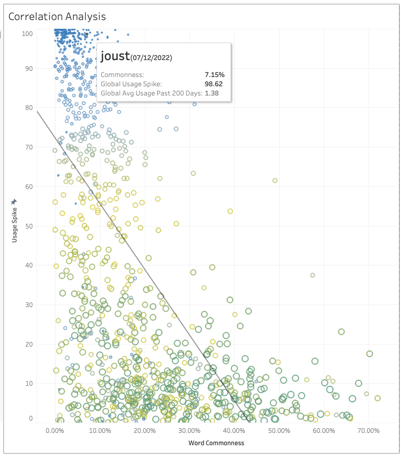
📈 Observations
We looked at how search interest on the Wordle day deviated from historical averages, and how this correlated with word commonality.
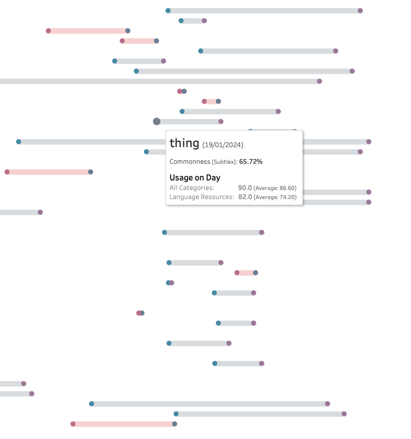
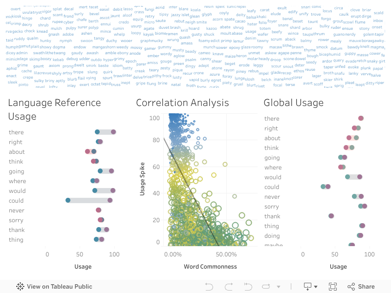
1. Wordle Day vs 200-Day Avg (Language Category)
We plotted this as a barbell chart, sorted by commonality.
Gray bars: Positive spike
Red bars: Negative spike
What stood out:
The more common words had little deviation — some even declined slightly. (red bars)
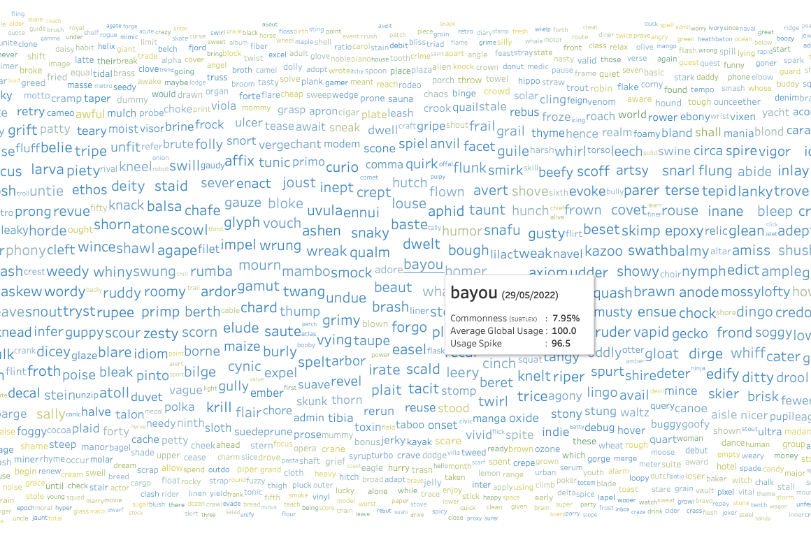
The less common a word, the larger the spike.
Words like “waltz” or “droop” showed huge increases (up to 100 on the trend scale).
Overall, the hypothesis holds — though the correlation is stronger in the lower half (less common words).
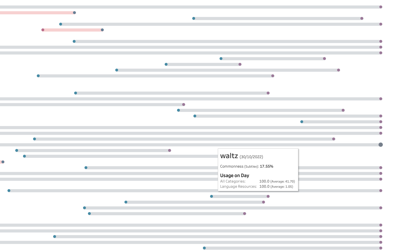
2. All-Categories Trend Comparison
This was similar to the previous view but covered all search categories, not just “Language Resources”.
The same pattern held.
Common words again showed muted or no change.
Rare words stood out clearly with search spikes.
This makes sense — common words are likely searched across many contexts, so Wordle adds only a small blip.